Regression Algorithms - Linear Regression

---

Introduction to Linear Regression

Linear regression may be defined as the statistical model that analyzes the linear relationship between a dependent variable with given set of independent variables. Linear relationship between variables means that when the value of one or more independent variables will change (increase or decrease), the value of dependent variable will also change accordingly (increase or decrease).

Mathematically the relationship can be represented with the help of following equation −

Y = mX + b

Here, Y is the dependent variable we are trying to predict

X is the dependent variable we are using to make predictions.

m is the slop of the regression line which represents the effect X has on Y

b is a constant, known as the Y-intercept. If X = 0,Y would be equal to b.

Furthermore, the linear relationship can be positive or negative in nature as explained below −

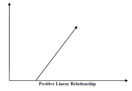
Positive Linear Relationship

A linear relationship will be called positive if both independent and dependent variable increases. It can be understood with the help of following graph −

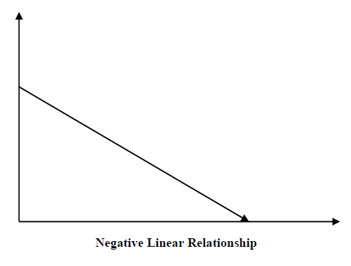
Negative Linear relationship

A linear relationship will be called positive if independent increases and dependent variable decreases. It can be understood with the help of following graph −

Types of Linear Regression

Linear regression is of the following two types −

• Simple Linear Regression
• Multiple Linear Regression

Simple Linear Regression (SLR)

It is the most basic version of linear regression which predicts a response using a single feature. The assumption in SLR is that the two variables are linearly related.

Python implementation

We can implement SLR in Python in two ways, one is to provide your own dataset and other is to use dataset from scikit-learn python library.

Example 1 − In the following Python implementation example, we are using our own dataset.

First, we will start with importing necessary packages as follows −

%matplotlib inline
import numpy as np
import matplotlib.pyplot as plt

Next, define a function which will calculate the important values for SLR −

def coef_estimation(x, y):

The following script line will give number of observations n −

n = np.size(x)

The mean of x and y vector can be calculated as follows −

m_x, m_y = np.mean(x), np.mean(y)

We can find cross-deviation and deviation about x as follows −

SS_xy = np.sum(y*x) - n*m_y*m_x
SS_xx = np.sum(x*x) - n*m_x*m_x

Next, regression coefficients i.e. b can be calculated as follows −

b_1 = SS_xy / SS_xx
b_0 = m_y - b_1*m_x
return(b_0, b_1)

Next, we need to define a function which will plot the regression line as well as will predict the response vector −

def plot_regression_line(x, y, b):

The following script line will plot the actual points as scatter plot −

plt.scatter(x, y, color = "m", marker = "o", s = 30)

The following script line will predict response vector −

y_pred = b[0] + b[1]*x

The following script lines will plot the regression line and will put the labels on them −

plt.plot(x, y_pred, color = "g")
plt.xlabel('x')
plt.ylabel('y')
plt.show()

At last, we need to define main() function for providing dataset and calling the function we defined above −

def main():
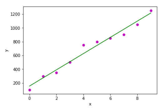
   x = np.array([0, 1, 2, 3, 4, 5, 6, 7, 8, 9])
   y = np.array([100, 300, 350, 500, 750, 800, 850, 900, 1050, 1250])
   b = coef_estimation(x, y)
   print("Estimated coefficients:\nb_0 = {} \nb_1 = {}".format(b[0], b[1]))
   plot_regression_line(x, y, b)
   
if __name__ == "__main__":
main()

Output

Estimated coefficients:
b_0 = 154.5454545454545
b_1 = 117.87878787878788

Example 2 − In the following Python implementation example, we are using diabetes dataset from scikit-learn.

First, we will start with importing necessary packages as follows −

%matplotlib inline
import matplotlib.pyplot as plt
import numpy as np
from sklearn import datasets, linear_model
from sklearn.metrics import mean_squared_error, r2_score

Next, we will load the diabetes dataset and create its object −

diabetes = datasets.load_diabetes()

As we are implementing SLR, we will be using only one feature as follows −

X = diabetes.data[:, np.newaxis, 2]

Next, we need to split the data into training and testing sets as follows −

X_train = X[:-30]
X_test = X[-30:]

Next, we need to split the target into training and testing sets as follows −

y_train = diabetes.target[:-30]
y_test = diabetes.target[-30:]

Now, to train the model we need to create linear regression object as follows −

regr = linear_model.LinearRegression()

Next, train the model using the training sets as follows −

regr.fit(X_train, y_train)

Next, make predictions using the testing set as follows −

y_pred = regr.predict(X_test)

Next, we will be printing some coefficient like MSE, Variance score etc. as follows −

print('Coefficients: \n', regr.coef_)
print("Mean squared error: %.2f" % mean_squared_error(y_test, y_pred))
print('Variance score: %.2f' % r2_score(y_test, y_pred))

Now, plot the outputs as follows −

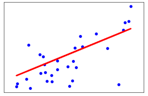
plt.scatter(X_test, y_test, color='blue')
plt.plot(X_test, y_pred, color='red', linewidth=3)
plt.xticks(())
plt.yticks(())
plt.show()

Output

Coefficients:
   [941.43097333]
Mean squared error: 3035.06
Variance score: 0.41

Multiple Linear Regression (MLR)

It is the extension of simple linear regression that predicts a response using two or more features. Mathematically we can explain it as follows −

Consider a dataset having n observations, p features i.e. independent variables and y as one response i.e. dependent variable the regression line for p features can be calculated as follows −

$$h(x_{i})=b_{0}+b_{1}x_{i1}+b_{2}x_{i2}+...+b_{p}x_{ip}$$

Here, h(x_i) is the predicted response value and b₀,b₁,b₂…,b_p are the regression coefficients.

Multiple Linear Regression models always includes the errors in the data known as residual error which changes the calculation as follows −

$$h(x_{i})=b_{0}+b_{1}x_{i1}+b_{2}x_{i2}+...+b_{p}x_{ip}+e_{i}$$

We can also write the above equation as follows −

$$y_{i}=h(x_{i})+e_{i}\:or\:e_{i}= y_{i} - h(x_{i})$$

Python Implementation

in this example, we will be using Boston housing dataset from scikit learn −

First, we will start with importing necessary packages as follows −

%matplotlib inline
import matplotlib.pyplot as plt
import numpy as np
from sklearn import datasets, linear_model, metrics

Next, load the dataset as follows −

boston = datasets.load_boston(return_X_y=False)

The following script lines will define feature matrix, X and response vector, Y −

X = boston.data
y = boston.target

Next, split the dataset into training and testing sets as follows −

from sklearn.model_selection import train_test_split
X_train, X_test, y_train, y_test = train_test_split(X, y, test_size=0.7, random_state=1)

Example

Now, create linear regression object and train the model as follows −

reg = linear_model.LinearRegression()
reg.fit(X_train, y_train)
print('Coefficients: \n', reg.coef_)
print('Variance score: {}'.format(reg.score(X_test, y_test)))
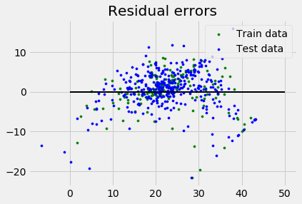
plt.style.use('fivethirtyeight')
plt.scatter(reg.predict(X_train), reg.predict(X_train) - y_train,
   color = "green", s = 10, label = 'Train data')
plt.scatter(reg.predict(X_test), reg.predict(X_test) - y_test,
   color = "blue", s = 10, label = 'Test data')
plt.hlines(y = 0, xmin = 0, xmax = 50, linewidth = 2)
plt.legend(loc = 'upper right')
plt.title("Residual errors")
plt.show()

Output

Coefficients:
[
   -1.16358797e-01  6.44549228e-02  1.65416147e-01  1.45101654e+00
   -1.77862563e+01  2.80392779e+00  4.61905315e-02 -1.13518865e+00
    3.31725870e-01 -1.01196059e-02 -9.94812678e-01  9.18522056e-03
   -7.92395217e-01
]
Variance score: 0.709454060230326

Assumptions

The following are some assumptions about dataset that is made by Linear Regression model −

Multi-collinearity − Linear regression model assumes that there is very little or no multi-collinearity in the data. Basically, multi-collinearity occurs when the independent variables or features have dependency in them.

Auto-correlation − Another assumption Linear regression model assumes is that there is very little or no auto-correlation in the data. Basically, auto-correlation occurs when there is dependency between residual errors.

Relationship between variables − Linear regression model assumes that the relationship between response and feature variables must be linear.